Control Theory Basics¶

2024 October 22/23 (2.5 hours)

Introduction¶

Control theory is probably the most important subject in FRC programming, and one you should consider a top priority. It is what separates well-performing robots from those that fail early. Contrary to what many people assume, what a robot design should aim to optimize for first is reliability, instead of speed and function. At Titan Robotics, it is our curse to overengineer solutions that do more than we can reasonably achieve, leading to barely any time for electrical and programming to test before the first competition and cause unforeseen mechanical issues in production. In their yearly strategy presentations, team 1678 (Citrus Circuits) consistently advises other teams to stick to tested solutions even if that means missing out on strategic advantages, as they often illustrate this by discouraging teams to use swerve drive without long-term experience with it. Mechanical, electrical, and programming all share the same goal—maximizing reliability. And so, on the programming side, this is how it is done.

The Problem¶

The biggest obstacle in robotics, which prevents us from completely solving every mechanical and programming problem, is noise. In practice, any mechanical system will have a variable amount of bending, twisting, slack, and other often unwanted forms of temporary deformation in rigid objects. This is also a unique aspect of FRC when comparing to other high-school level robotics programs. Many material properties start to show significantly at lengths and masses of the FRC size, unlike the more compact FTC and VEX robots. Simple contraptions, like measuring tape as a robot mechanism (used by teams in the 2020 FTC competition), would not work in FRC because of reliability criteria. At such scale, you want to manuever the robot while adapting to undesirable physical changes.

What is Control Theory¶

Open-Loop vs. Closed-Loop¶

Control theory is a field of applied mathematics regarding optimizing control systems for accuracy and response time. There are two types of control: open-loop (feedforward) and closed-loop (feedback). As the names suggest, open-loop control utilizes inputs to determine an output without considering the output. Closed-loop control utilizes output back into the system, hence its second name “feedback”. An example of an open-loop system is boiling water on a gas stove for a certain time. The gas stove only cares about the volume of gas that the user selects, and does not care about whether or not the water is boiling or what the temperature of the water is. Temperature-regulating air conditioners and HVAC systems are an example of a closed-loop system: the temperature is fed back into the control system to determine the new output, eventually adjusting the room to the desired temperature.

There are many systems that depend on closed-loop control to function. Reliably controlling DC motors to be at certain rotational speed is not possible without taking into account its rotational output measured by an encoder. The motor controller uses this value to compute a close-enough voltage to feed into the motor.

PID Controllers¶

PID (proportional–integral–derivative) controllers are the most common form of adjustable closed-loop controllers. It allows you to tweak three constant coefficients (as stated by its name) to increase efficiency and response while lowering undesirable effects like undershooting or overshooting.

Imagine you are trying to drive a car to a location on a straight but slippery and poorly constructed road. Call your destination’s location \(r(t)\) (also called the setpoint). At time \(t\), you know that your car is located at \(y(t)\). These are the two variable inputs to the PID controller. The process variable, \(e(t) = r(t) - y(t)\), is the difference between the destination and the car’s current position.

The constant inputs to the PID controller are \(K_p\), \(K_i\), and \(K_d\), three coefficients that go into the equation \(u(t) = K_p e(t) + K_i \int_0^t e(\tau)\,d\tau + K_d \frac{de(t)}{dt}\), where \(u(t)\) is the distance that we tell the car to go at time \(t\). (It isn’t too important to understand this math.) We send \(u(t)\) to the motor, and wait until we figure out where the car is after we tried to drive \(u(t)\). Then we repeat this process.

../../_images/PID_en.svg — The basic idea of a PID controller¶

The effect of changing \(K_p\), \(K_i\), and \(K_d\)¶

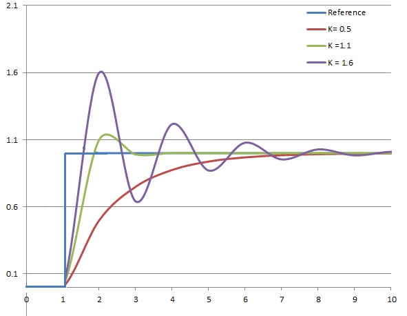
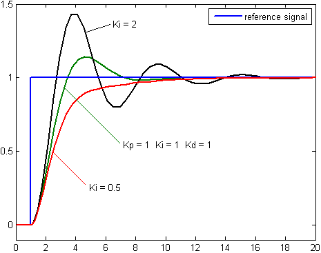
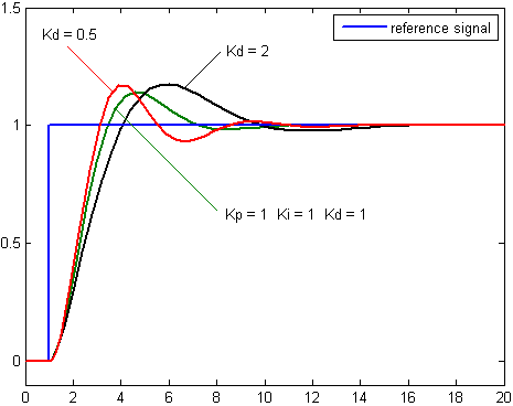
Say we want to drive our car to the campground 1 mile down the road. We use a PID controller to control the acceleration of the car, but we don’t know the optimal \(K_p\), \(K_i\), and \(K_d\), so we try driving our car using the PID controller a few times.

This is what happens when we change \(K_p\):

This is what happens when we change \(K_i\):

This is what happens when we change \(K_d\):

In general, we usually set \(K_i = 0\), and we manually tune \(K_p\) and \(K_d\). None of these constants should usually be significantly more than 1.0, as that tends to cause drastic overshooting.

NOTE: Another less-regarded factor in PID loops is data frequency. Since it’s a discrete model, lower delta time results in better calculations.

Using the PID controller on the robot¶

There is a PID controller implemented in every Falcon 500 motor. Every output on the robot—this being the swerve drivebase wheels and rotators, the arm, the elevator, etc—should ideally go through a PID controller with correctly tuned PID constants. The math behind it isn’t necessary to learn to use one, but this article on the WPILib documentation explains it well. WPILib includes a PIDController class implementation for general use.

PID with feedforward¶

Sometimes it is beneficial to add a feedforward component to a PID control system to compensate for variables in specific circumstances. We utilized PIDf in our old swerve subsystem code to account for friction. In practice, the implementation is incredibly simple. Add the desired amount of feedforward output multiplied by a coefficient to the PID output. This WPILib article shows PIDf in practice.

Exercise 1 - Tuning a PID controller¶

See an interactive example here that shows a circle attempting to position itself under the cursor. Here is another interesting website that shows a simulation of a cart balancing an arm by changing its velocity using PID. There are many strategies for tuning PID, but this is the one I have bookmarked and use for FRC.

Exercise 1: Try to tune the PID constants of the first example for optimal behavior.

Exercise 2 - Using PID in Java¶

Overview¶

The simulation includes a gravity-affected elevator that can be controlled through its acceleration. For this assignment, your goal is to pass the target position and target velocity through two PIDController class instances (each should have their own) with well-tuned parameters. The result should use the PID controller implementation to make the elevator as responsive as possible. Manually adjust the values until results are satisfactory.

The PID implementation is identical to the one from WPILib. Create a new class instance and use the first three arguments as your PID parameters. The class has a method called calculate that will provide you with the PID output. Set the derivative of the value you’re trying to reach as this output.

// Pseudo code
value_derivative = pid.calculate(measured_value, target_value);
acceleration = pid.calculate(measured_velocity, target_velocity);

Only the elevator.setMotorAcceleration method will actually control the elevator. elevator.setTargetVelocity and elevator.setTargetPosition are what you should use in your PID calculations. Here are all available elevator methods. All unites are arbitrary.

getInput: from -1.0 to 1.0, use left and right arrow keys
getMotorAcceleration
getTargetVelocity
getTargetPosition
getAcceleration
getVelocity
getPosition
setTargetPosition
setTargetVelocity
setMotorAcceleration

Installation¶

Clone the Training2024 repository and checkout into the control-theory-template branch.

Code¶

All relevant code should be written inside ElevatorPlayground.java. start and update methods are provided to control the elevator.

Hints (what we did during the lesson)¶

Setting up the velocity PID and binding it to the left/right keys¶

This sets up the velocity PID to try to attain the speed specified by the arrow keys (no keys pressed = 0 m/s, right key pressed = 1 m/s, left key pressed = -1 m/s).

ElevatorPlayground.java¶

import sim.Elevator;
import sim.PIDController;
import sim.PlaygroundBase;

public class ElevatorPlayground extends PlaygroundBase {
    private PIDController velocityPID = new PIDController(40, 0, 0.3);
    /**
     * This function runs once on the first frame. (like `-init` in WPILib)
     */
    @Override
    public void start(Elevator elevator) {
        elevator.setMotorAcceleration(0);
        elevator.setTargetVelocity(0);
        elevator.setTargetPosition(0);
    }

    /**
     * This function runs every frame. (like `-periodic` in WPILib)
     */
    @Override
    public void update(Elevator elevator) {
        elevator.setTargetVelocity(elevator.getInput() * 1);
        elevator.setMotorAcceleration(velocityPID.calculate(elevator.getVelocity(), elevator.getTargetVelocity()) + 9.8);
        System.out.println(elevator.getVelocity() + " error: " + (elevator.getVelocity() - elevator.getTargetVelocity()));
    }
}

Now, the task¶

The task is to make a position PID, in order to make the block go to position 1 m. If you’re stuck, use this template code:

ElevatorPlayground.java¶

import sim.Elevator;
import sim.PIDController;
import sim.PlaygroundBase;

public class ElevatorPlayground extends PlaygroundBase {
    private PIDController velocityPID = new PIDController(40, 0, 0.3);
    // You need to tune the position PID yourself
    private PIDController positionPID = new PIDController(1, 0, 0);
    /**
     * This function runs once on the first frame. (like `-init` in WPILib)
     */
    @Override
    public void start(Elevator elevator) {
        elevator.setMotorAcceleration(0);
        elevator.setTargetVelocity(0);
        elevator.setTargetPosition(0);
    }

    /**
     * This function runs every frame. (like `-periodic` in WPILib)
     */
    @Override
    public void update(Elevator elevator) {
        elevator.setTargetVelocity(/* Use the position PID to figure out the target velocity here */);
        elevator.setMotorAcceleration(velocityPID.calculate(elevator.getVelocity(), elevator.getTargetVelocity()) + 9.8);
        System.out.println(elevator.getVelocity() + " error: " + (elevator.getVelocity() - elevator.getTargetVelocity()));
    }
}

Challenge¶

Start only after completing the main task

For this challenge, your goal is to tune the PID parameters automatically. Use any method you want to optimize the three PID coefficients by minimizing the residual between target and real positions of the stick.

More On Robot Control¶

CW: long yapathon ahead

The Problem: In Practice¶

A common example of affected software input is when you introduce an encoder to measure axis position. There are several factors that will impact your readings: wheel and belt slippage, friction, gearbox slack, misalignment of the sensor itself, and many other factors. Then when you want to output a signal to a motor, such as one controlling an arm, you have to deal with more factors: gravity, variable friction of the system, variable arm weight that affects torque, and many more. These physical factors often cannot be calculated because of their complexity and noise. Since it is impossible to make the perfect encoder measuring system, the best you can do is minimize those factors during the design process and account for them in software. If a system contains more than one rotating axis, the encoder should be placed on the axis closest to the output to minimize effect of gear slack. Belts can prevent this as they don’t require the same tolerances, but ideally the encoder should be placed in the most representative place of what you are trying to measure.

What Typically Happens¶

On the software side, the raw encoder output can (and often is already by your library) be filtered through various methods to separate the desired signal from the noise. We will cover some of these methods later. But ultimately, it is also important to direct robot output in such a way that accounts for physical aspects without the need to model unpredictable complexity. When you create a plan on how to program a rotating arm, the first instinct of us is to recreate a geometric model of the arm from the motor output. We are used to drawing diagrams and solving problems through simulations in physics and math classes at IMSA and previously. But the real world is too complex for inverse kinematics based on torque equations to be accurate enough. Some of these equations weren’t even defined for ranges of values appearing in production. Although theoretical models are still very applicable in FRC, many systems used in FRC are hard to describe using these theoretical models, or have so much potential for error that the theoretical model won’t accurately predict how the system will be have in the real world. Combining those models with control theory methods for reducing the impact of noise (such as adding a PID controller as the last step) leads to great results.

Design Decisions First¶

More often than not, the simplest solutions are also the best, most reliable. Going back to the arm programming example, it is important to consider all constraints and criteria of the problem. Removing unnecessary functionality is one way to approach it. Does your arm need to move to any position in its degree of freedom? Does it need to do so with speed, precision, accuracy, while holding a heavy object, without causing too much acceleration? Perhaps you may only need to move it to three total positions throughout the entire game? If so, maybe an elevator system would actually be a more suitable mechanism as it only has one degree of freedom with higher rigidity. Programming an elevator, which consists of a pulleys with a motor or two, is significantly easier than programming a rotating arm affected by gravity. It is more energy efficient too as it won’t require as much current draw to counter gravity with motors (another factor that needs higher consideration: less subsystem power usage means a faster drivebase). In this case, your first action should be to run to the nearest design member and ruin their dreams of attaching a custom 5-axis arm to the swerve drivebase.

Implications of Complexity¶

Although, sometimes you might have to be stuck with programming a rotating arm. In which case, you can predetermine the necessary motor values beforehand. Create a table for the arm to be static at a certain angle and also that angle but with a weighted object. It seems simple in theory, but once you realize that the battery voltage affects motor output, the problem gets exponentially more difficult. Now imagine if you still decided to stick with your old inverse kinematics equation. Your equation would now have to consider battery strain, on top of drivebase movement and other factors. And now, consider this but with the typical occurrence: you only have two hours a week to test it and competition is coming up. What about other subsystems? You have code for them too and you need to test it (your drivebase code should be consistent over the years for this reason). Well, what if the member who singlehandedly wrote the arm subsystem and every command for it gets sick? It is far simpler to debug a close-enough estimation of the real world than complex equations that model it.

But this section is an exaggeration: most FRC teams do not encounter every possible negative outcome in one season. Simply, it is to state that robot design and programming should account for unforeseen challenges. The pandemic has taken a toll on this team as significant amount of knowledge and connections have been lost. But with each season, there are improvements. The arm example is a retelling of the events that occurred during the 2022-2023 FRC season when our knowledge regarding creating reliable designs and writing reliable code was limited. I encourage reading ChiefDelphi posts for the purpose of regaining these skills. What separates consistently well-performing teams and everyone else is proper documentation and long-term connections.